Reading Serial IMU Data

Last time we left off, we were able to send data serially to our python client which in turn, published the data to our ROS topic. Since we made a proof of concept (POC) with static values, we should be able to use this functionality to send the data of the Inertial Measurement Unit (IMU) serially. One known thing about IMU's is they are notoriously noisy so the readings from the accelerometer and gyroscope need to be filtered in order to observe meaningful data. Below we will explore one way to read IMU data serially, run it through a complimentary filter, and write to the output buffer.

Reading the IMU

If you remember from an earlier blog post where I listed the sensors I bought, the IMU is a LSM6DS33 3D Accelerometer and Gyro. It includes a 3.3V voltage regulator that allows a range of 2.5. to 5.5V which is nice since the Arduino Pro Mini pulls 5V. Pololu, the website where I purchased the sensors, has a resources section which directed me to a library specifically written for the sensor. Upon reviewing the source on GitHub, I decided this would be a good way to expedite development since the library is very simple and I have no experience reading analog values. After installing the library, an example sketch can be loaded through the Arduino IDE menu.

                       

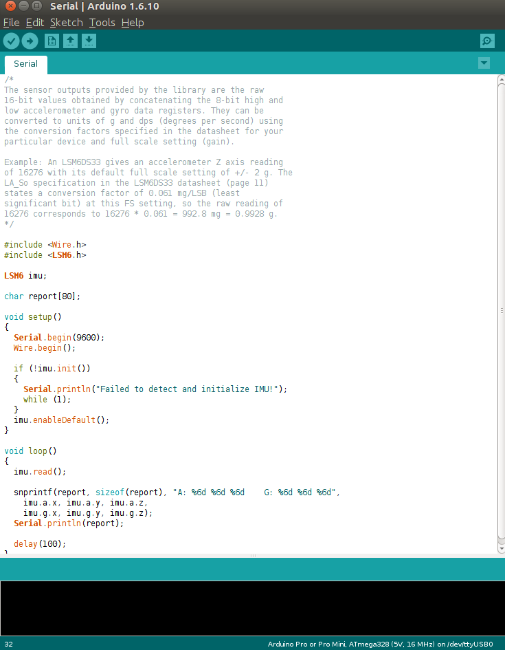
The code on the right is the LSM6 Sketch and it contains everything you need in order to read the data from the IMU. All you need to do now is upload this sketch to the Arduino, make sure the IMU is connected correctly to the Arduino, and to provide power. While the program is running, if you have the serial monitor open, you will see a stream of data filling the screen with readings.

(Note: The stutter in the readings is caused by the Serial Monitor and not the sensor as we will see later when our ROS topic is publishing data in real time without lag.)

Interpreting the Data

The above image shows readings that are not very intuitive at first glance and can scare new hobbyists, hopefully the explanation below will help demystify the numbers and process.  

Accelerometer

The expected values for the accelerometer are X = 0, Y = 0, Z = -1 which just means that there is a downward force of 1 G. For those that might not find the above expected values intuitive, there are two reasons we are expecting these values. First, gravity is always acting, causing us to fall towards the center of the earth (1 G Force or -9.8 m/s^2). Second, since we are modeling the real world the sign (+-) of the Force really only determines the direction the Force is applied. For example, the Z axis represents up(+) and down(-). The accelerometer can also measure different scales of forces but in our case we have set the full scale setting to 2 which means we can effectively measure forces between -2G and 2G.

Now that we have expected values, we can begin to convert the raw readings into actual Forces. Looking at the image above we can take a random value from the 3rd column (Z acceleration force); I will pick -16,642. From page 15 of the LSM6 Data Sheet, we can find the units for the full scale setting of 2, linear acceleration sensitivity, 0.061mg/LSB (milli g's / Least Significant Bit). Taking the raw data and multiplying the sensitivity ratio we get the following:

1. -16,642 * 0.061 = -1,015.162 mg (These units are milli g's)

We need to account for the milli g's by dividing the number by 1000 to get g units.
2. -1,015.162 mg / 1000 mg = -1.015162 g

This value is close enough to -1 that we can dismiss the extra force measured as background noise. The above math can be made more generic so it can be applied to each dimension measured by the accelerometer.

3. Raw Data * Linear_Acceleration_Sensitivity * (1 g / 1000 mg)

If we convert the Linear_Acceleration_Sensitivity value from millig's to g's during setup we can reduce total calculations per iteraiton.

4. Raw Data * Linear_Acceleration_Sensitivity_G = result
(Note: Steps 1 & 2 combined are Step 4)

Gyroscope

The expected values for the gyroscope at rest are 0 dps (degrees per second) for X, Y and Z dimensions because the gyroscope measures the rate of change in angular acceleration. The raw data is measured in mdps/LSB and must be converted in order to be a meaningful value. Again, looking at page 15 of the LSM6 Data Sheet, we can find the angular rate sensitivity for the full gain setting 245 which is 8.75mdps/LSB. (milli degrees per second / Least Significant Bit)

First our angular rate sensitivity is in mdps and we need to turn it into dps.

1. 8.75 / 1000 = 0.00875 dps/LSB (This result is the Angular_Rate_Sensitivity in terms of g's)

Multiply the raw value by the angular rate sensitivity to get degrees per second

2. Raw Data * Angular_Rate_Sensitivity = result

If we calculate some of the values in the above image, we will notice that the results are not 0 and in fact they oscillate between a specific range. This oscillation is due to imperfections in the sensor and must be accounted for by setting a threshold that floors the readings and helps remove the noise. In our case, I checked the data sheet and noticed there is a rate of (+-)10 dps so any readings between -10 and 10 are floored to 0.

Note: The result is in degrees per second but we are reading data from the IMU much quicker than 1 second intervals. To remedy this we need to integrate (sum the data over time) the result by multiplying by the time it took to run the last iteration (delta time [normally in milliseconds]). As soon as we integrate the gyro data (gyroData * dt), we introduce error because our sample size is not continuous which will cause error interpreted as drift; the main reason why we will smooth the data using a complimentary filter.

Complimentary Filter

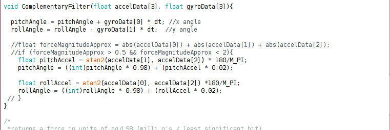
The idea of smoothing out the data is not new and there is even a standard call the Kalman Filter. While the Kalman Filter is very complex, there is a simpler approach that requires little overhead. (We will be implementing a Kalman Filter in the future, just not right now.) For now, we will use what is called a Complimentary Filter:

angle = (angle + gyroData * dt) * 0.98 + (angle of acceleration * 0.02) 

To get the angle of acceleration we can use the arc tangent but this causes problems because quite frequently our divisor will be 0 and we cannot divide by 0. Luckily we have access to the atan2 function which allows us to supply 2 inputs and get an angle representative of the inputs. There are plenty of websites that will explain what the arctangent and atan2 functions are so if you are interested I suggest reading further. 

(Note: The above code will probably not work copy pasta unless the rest is configured exactly the same.)

(Disregard the linear values as they are debug terms I am using)

We see that at rest the IMU is reading 0 and when disturbed, we get precise readings. Moving forward these values will be fed into a PID controller which will be used to stabilize and move the quadcopter.

Findings

There is very little documentation for hobbyists online at the moment and I am continually scouring the internet for resources but they are far and few between. I think this will be a good opportunity to add to the collective knowledge base of the internet with my findings and hopefully my struggles will make someone else's experience easier. As always, feel free to leave a comment or question. Happy flying!